Linux Kernel 2.6.29 + tux3

In this section we are going to explore a certain version of the Linux Kernel, the tux3 branch from March 14, 2009. This version contains the Linux tree up to March 10. The 2.6.29 was released on March 23 so this is not exactly the final version. I picked it because it contains btrfs and, at the time of writing this report, it is the latest one that was published by Daniel Phillips, the creator of the tux3.

The rest of this section is made up exclusively of figures accompanied by extensive captions.


Map of the external symbols. This plot shows the external symbols for 55 kernel modules from the tux3 git repository. Each tick represents an external symbol. The file systems are show in alphabetical order. The big compact chunks of external symbols related to jbd and jbd2 are visible for ext3 and ext4. The fact that ocfs2 is also making use of jbd2 is also noticeable. Later in this section we will see how this representation looks when is reorganized based on similarities between file systems.

Number of external symbols. This plot shows the ranking of the file systems based on the number of external symbols. We can see that the range is about 300 symbols and there are no sudden jumps: some sizes are more popular than others but overall the space is filled quite smoothly.

Number of external symbols by categories. This is the same plot as the previous one except this time the file systems are grouped in categories.

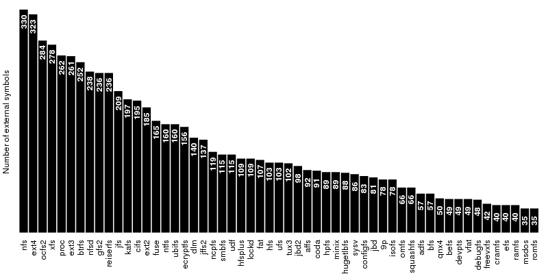
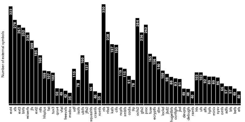
The first group, which contains the disk-based file systems, is led by ext4 which is ahead of xfs by 45 external symbols. Note that the number of external symbols for both ext4 and ext3 is boosted by the fact the journaling part not implemented internally but provided by jbd2 and jbd respectively. At the other end of the scale is a group of 4 file systems out of which only two, freevxfs and qnx4 are truly self-contained. The other two, msdos and vfat are getting most of their functionality from the fat module which is more than twice of their size.

The second group contains the file systems dedicated to optical mediums and it holds no surprises: udf is ahead of isofs by a comfortable margin.

The same thing is also true for the the third group, of the flash-based file systems, where the first place is taken by ubifs followed by jffs2. The third placed is secured by squashfs while the bottom is shared by cramfs and romfs which are separated by only 5 symbols.

The fourth group is the one dedicated to the network file systems. Here the first two spots are taken by nfs and nfsd, which provide kernel support for NFS client and NFS server. On the next two places, at very close distance between them, are kafs, the Andrew File System, and cifs. The end is shared by coda and 9p.

The fifth group contains, in this order, the only two cluster-based file systems: ocfs2 and gfs2. The number of external symbols for ocfs2 is increased due to the use of the jbd2 journaling library.

The sixth group, the one dedicated to memory-based file systems is dominated authoritatively by proc which has almost 100 more external symbols than fuse, the file system from the second place. As expected, at the bottom sits ramfs.

The seventh and last group is dedicated to ancient file systems. The first place is shared by hfs and ufs. Quite surprising, this is only one of the three ties in this group, the other two being hpfs/minix and adfs/bfs.

The 50 most popular external symbols. The symbols are sorted in the descending order of their frequency while the file systems are sorted in the descending order of number of external symbols they use.

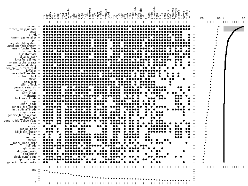
The first two symbols are used by the function tracer. On the third place we have a tie between kfree, which is used by everybody except by ramfs, msdos and romfs, and kprintf which, surprising, is avoided by vfat, ramfs and msdos.

As expected, the kmem operations are among the most popular one. So are the some basic operations like strlen, memcmp and strsep.

Another thing we can notice are some (expected) pairs of calls that are always used together: register_filesystem/unregister_filesystem, _spin_lock/_spin_unlock and kmap/kunmap.

Another (again expected) observation is that the lack of (un)register_filesystem identifiers in the modules which only provides services to others: dlm, lockd, fat, and jbd2/jbd2.

Heatmap of the Hamming distances. If we think of each file systems as a string of bits with one indicating the presence of a certain external symbol and zero as the absence of it then the Hamming distance is the minimum number of substitutions necessary to change one string into another. The heatmap is symmetric. The red indicates a Hamming distance of zero, which corresponds to maximum similarity, and yellow indicates very little similarity. Everyone is similar with itself so the diagonal is red. In this plot the file systems are sorted in ascending order of their number of external symbols. What we are going to do next is to reorder the rows and columns in a way that brings closer the file systems that are similar.

Hierarchical clustering. As the name implies, hierarchical clustering builds a hierarchy of clusters. There are two ways to do this: one is to start from bottom, with all the data points as clusters and then, at each step, merge two of them. This is also know as agglomerative nesting. The other one is called divisive and starts from top, with everything in a big cluster, and at each steps performs a split.

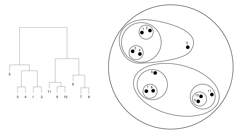
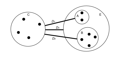
Below is an example of clustering 11 points situated in a 2D plane. Left is a dendrogram, a tree diagram usually used to represent the result of a hierarchical clustering. Right is a representation using nested clusters.

Single linkage. When all the clusters only contains one point we can easily define the distance between them as the distance (d) between the respective points. After each merge operation we need a way to define the distance (D) between this new cluster and all the old ones. One way to do this is to consider the distance between two clusters as the minimum distance between any pair of nodes with one node in a cluster and another one in the other. Formally we could express this as D(A,B) = { min(d(x,y)) | x ∈ A and y ∈ B }.
This method is best suited for constructing elongated clusters like the ones below.

Complete linkage. In this case the distance between clusters is defined as the maximum distance between the pairs of nodes which contain one node from one cluster and one from the other. Similar with the previous case, this could be express as D(A,B) = { max(d(x,y)) | x ∈ A and y ∈ B }. This method is capable of creating small and compact clusters.

Group average. We can also define the distance between two clusters in such a way that all the pairwise distances contribute to the result. If we take the average of all the pairs then the method is called group average.

Ward's method. This method works like this: for each cluster we compute the sum of squared deviations from the cluster's centroid. Then we sum up all these sums and get a total error sum. At each step we merge the two clusters which minimize the increase of total error sum.

McQuitty's method. In this method, after each merge, the distance between the new cluster and the old ones are computed based on the distances of the two clusters that were merged. In the example below, two clusters, A and B, were merge and formed a new cluster E. The distance D3 between E and another cluster C is defined to be D3= (size(A)×D1 + size(B)×D2)/(size(A) + size(B)). This method is also call WPGMA (Weighted Pair Group Method with Arithmetic Mean).

Clustering using the Hamming distance and Ward's method. Let's now take a look at how the heatmap of the Hamming distances we introduced earlier looks like when we reorder it using Ward's algorithm. The most noticeable thing is the distinctive division of the map the due to nfs/proc and nfsd. Many things are clustered in expected ways: the ext2/ext3/ext4 family (lower left corner), the coda/smbfs/ncpfs network file systems, the jbd/jbd2 journaling services.

Dendrogram of the clustering using Hamming distance and Ward's method. If we look only at the dendrogram we can notice that this method divided the file systems in two big parts: complex disk-based systems including cluster file systems (which contain a disk-based part inside them), and everything else. We can also observe that most of the ancient file system category is contained almost completely in one big branch (fatminix). Some unusual matches: 9p is situated quite far from the rest of the network file systems and tux3 ends up keeping company to the group of ancient file systems. In contrast, btrfs enjoys the neighborhood of xfs and gfs2 in the upper class of complex file systems.

Clustering using the Hamming distance and complete linkage. Unlike the previous method, the rearrangement using the clustering based on furthest neighbor strategy (also known as complete linkage) creates a heatmap with a nicely defined center. The kernel is formed by a group of ancient file system and a few memory-based file systems. In the lower left we can also notice a close-knit group formed by ext2/ext3/ext4, ocfs2 and reiserfs. As before, a few classic modules, jbd/jbd2 and coda/smbfs/ncpfs, are again together.

Dendrogram of the clustering using the Hamming distance and complete linkage. Here we can see that the big nice split from Ward's method is replaced by a more scatter division. The complex disk-based file systems are now split in two parts, ocfs2ext3 and xfsubifs, the second of them being muddle by two flash-based file systems (jffs2 and ubifs). btrfs is again next to gfs2 and close to xfs but, surprise, also next to ntfs. Like before, tux3 is close to a bunch of ancient file systems. isofs, squashfs and cramfs, two read-only file systems are together from the start this time with romfs, the only other read-only file system, keeping a decent distance from them.

Clustering using the Hamming distance and group average. The group average method, usually used to identify bell-shaped clusters, generates a heatmap with a prominent off-center kernel. As in the previous case, this is made up of mostly by ancient file systems. Easily noticeable groups are again formed by the ext2/ext3/ext4, jbd/jbd2 and coda/smbfs/ncpfs.

Dendrogram of the clustering using the Hamming distance and group average. In this representation, the skew is also very visible. From a high-level perspective, we have a big cluster jbdubifs and a few small ones (ext4ext3, gfs2reiserfs and cifskafs) which are merged in the final merging steps with some file systems (nfs, btrfs, dlm, etc). The intuition behind this is that, as the file systems use more and more external symbols, they become more loosely connected.

Clustering using the Hamming distance and McQuitty's method. The heatmap in this case is somehow similar with the one from complete linkage.

Dendrogram of the clustering using the Hamming distance and McQuitty's method. If we ignore the skew induced by proc/nfsd/nfs and the fact that the complex disk-based file systems (xfsreiserfs and ocfs2ext3) are not sharing the same level, then the resulting tree is nicely split in similar things.

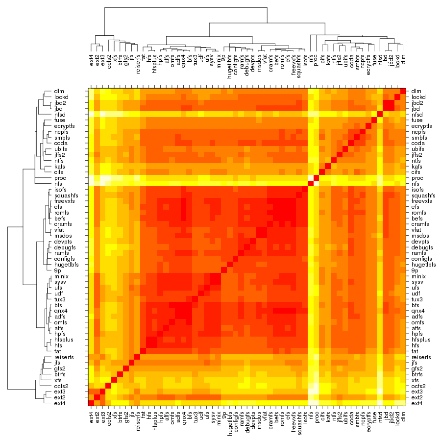
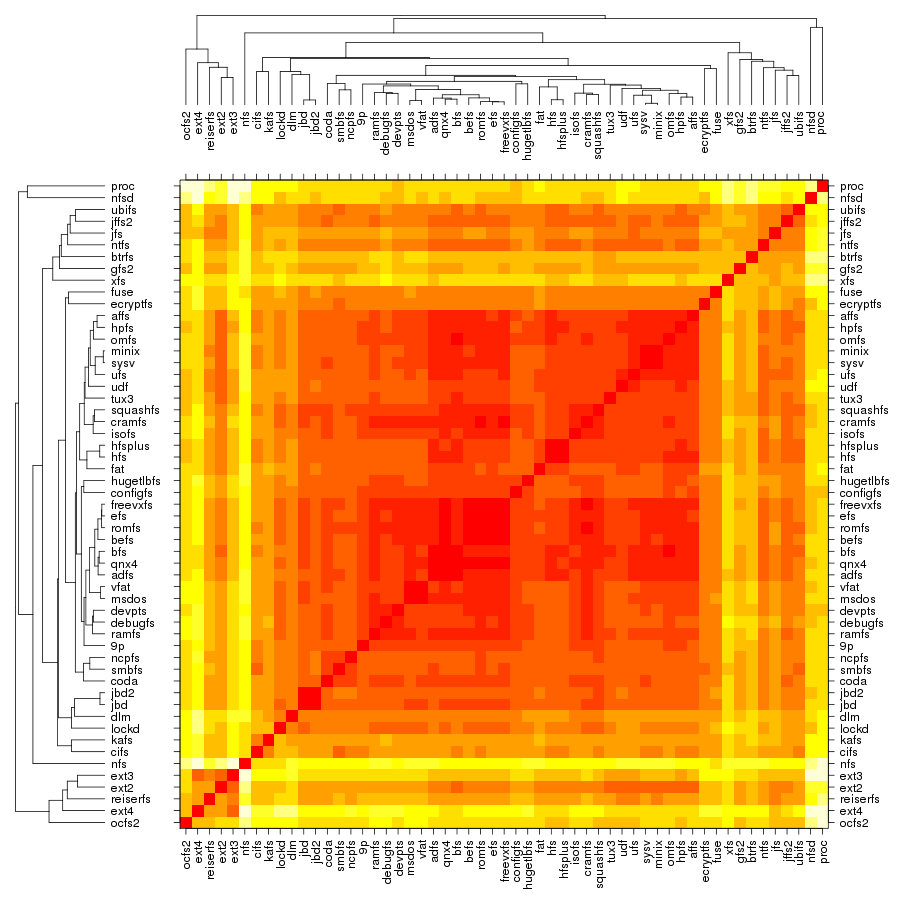
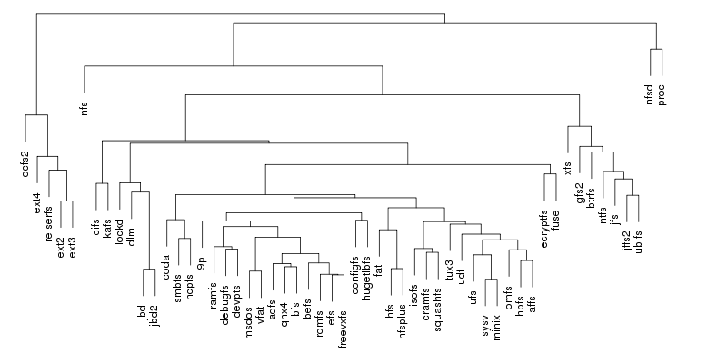
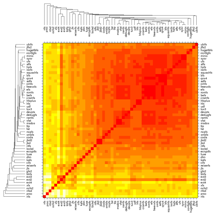
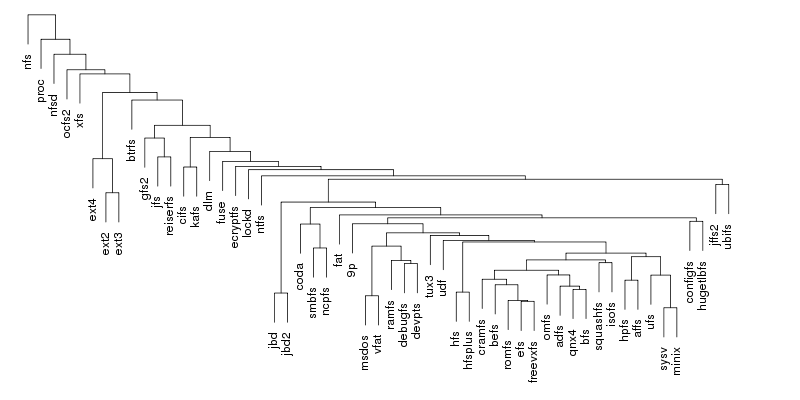
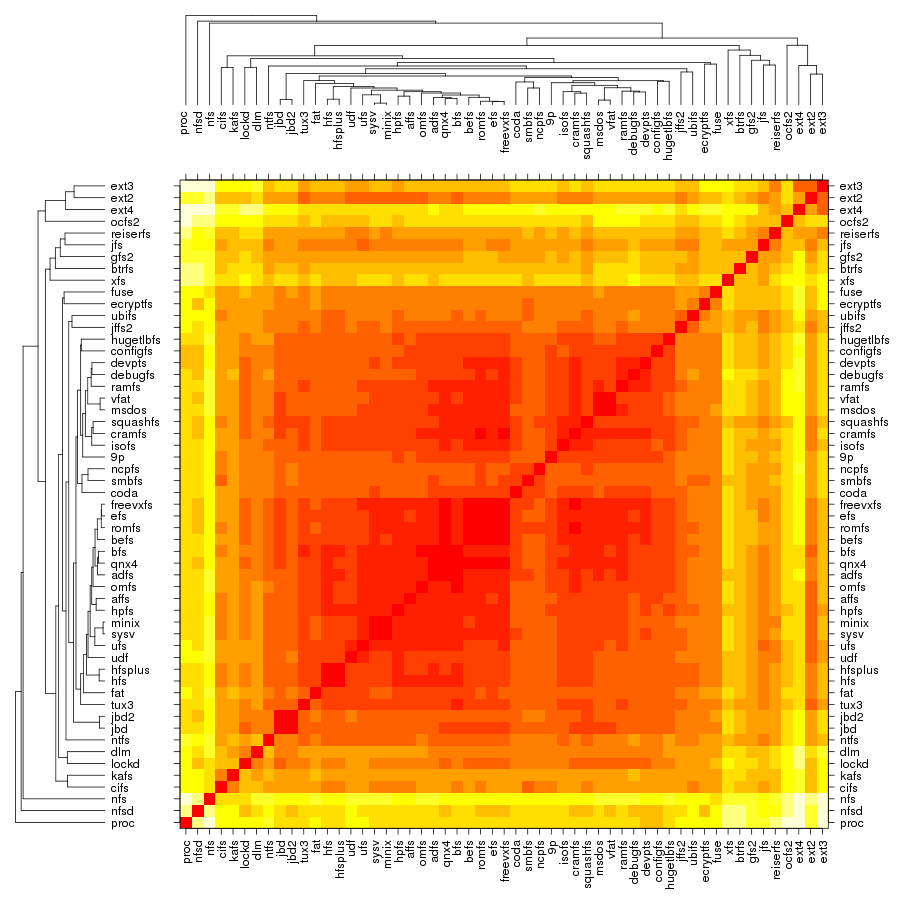
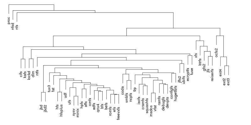
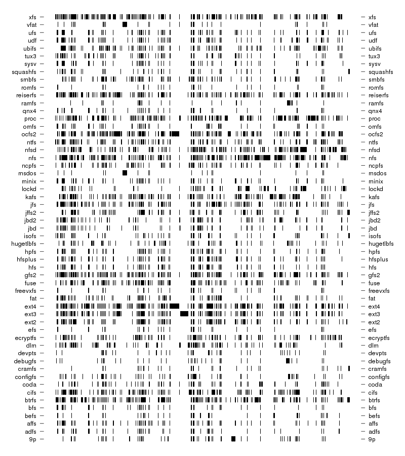
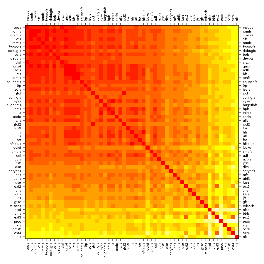
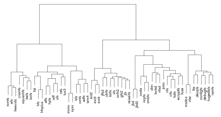
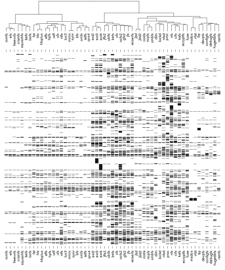
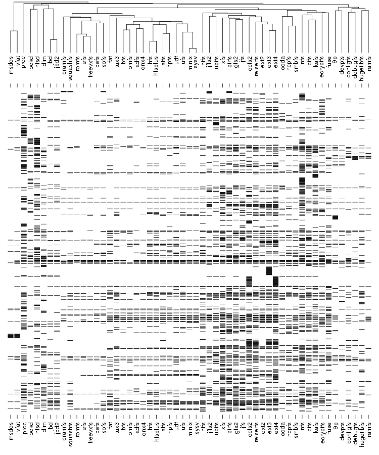
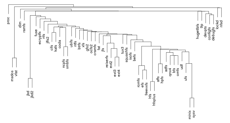
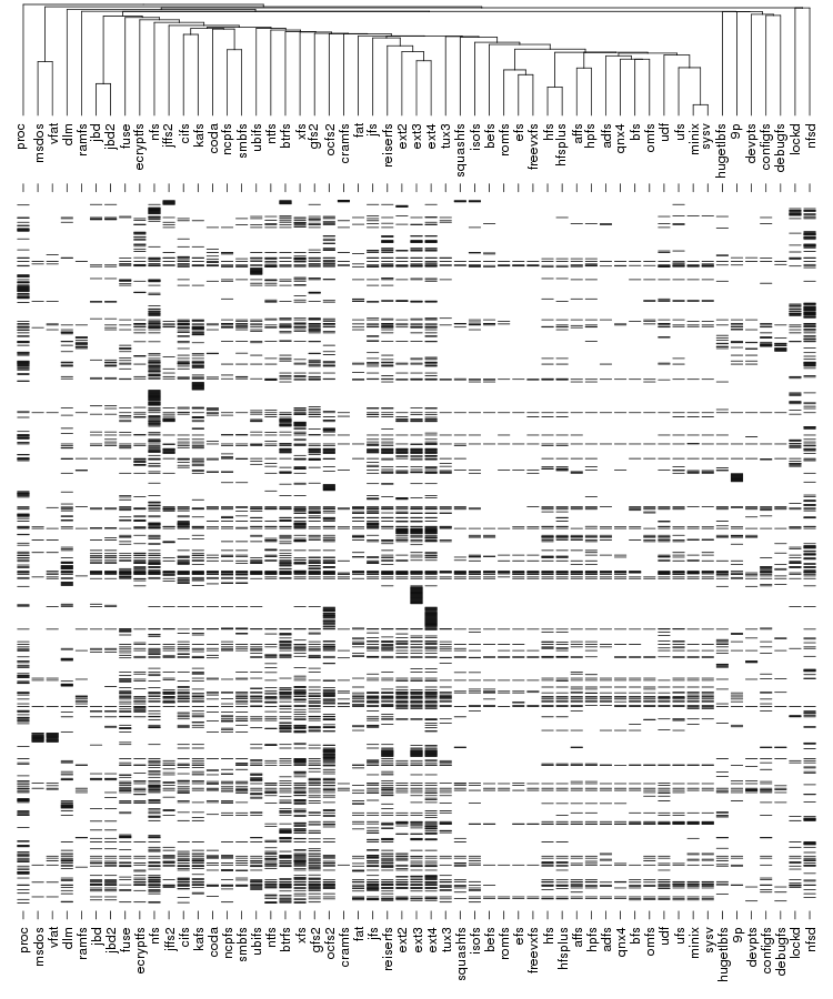
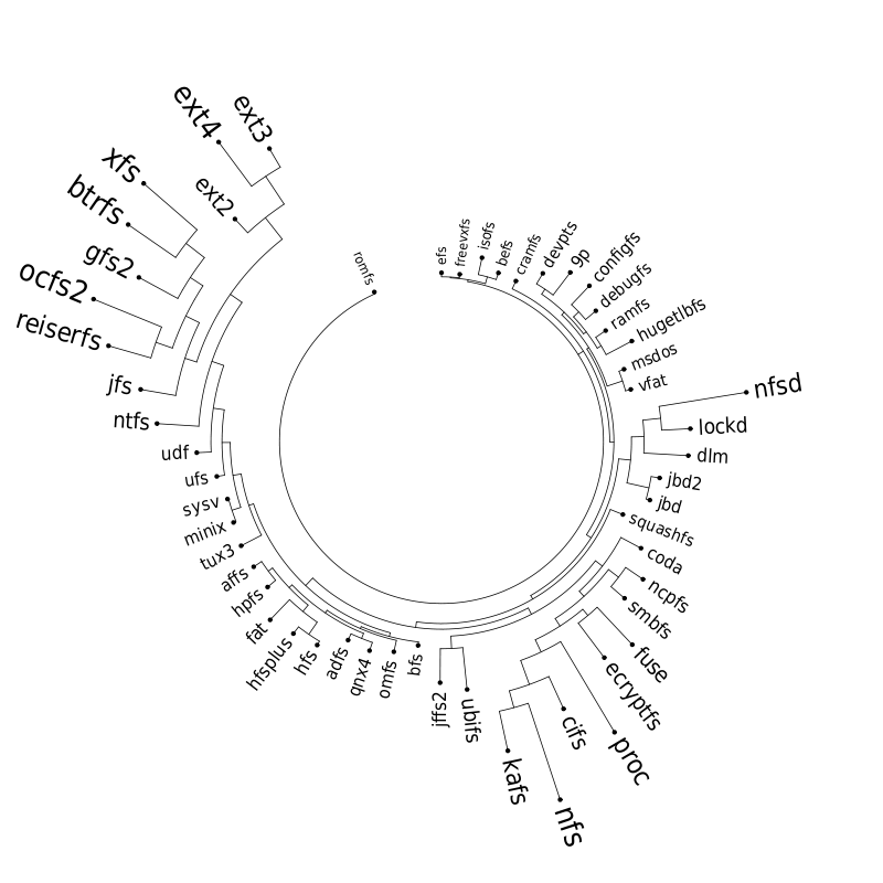
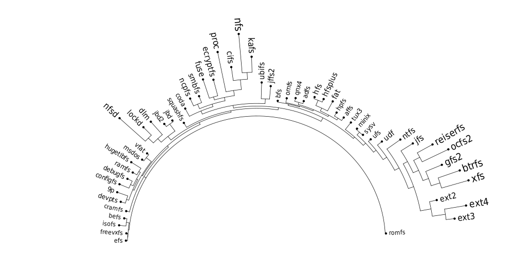
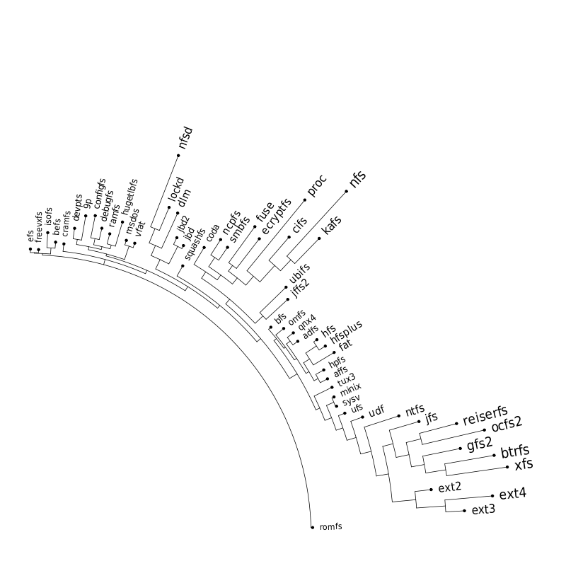
Following are a set of dendrograms using Canberra distance. In our case, this metric is equivalent with the number of different external symbols between two modules. After each dendrogram a reordered map of symbols is also plotted.


Phylogentic tree. Pars is a program that can construct an evolutionary tree which requires a minimum number of changes (maximum parsimony). The program is part of PHYLIP, a computational phylogenetics package created and maintained by Joseph Felsenstein.

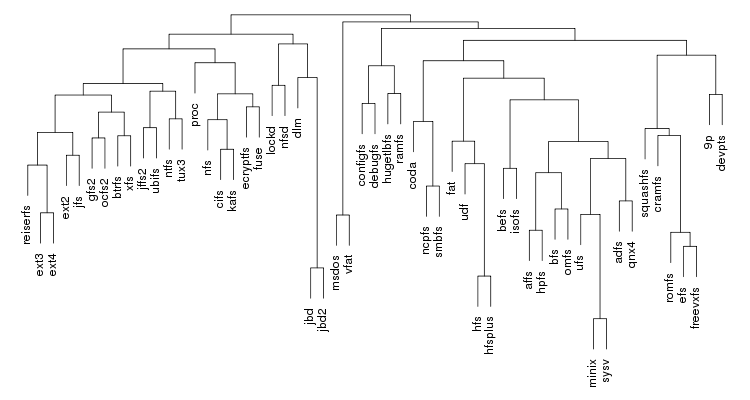
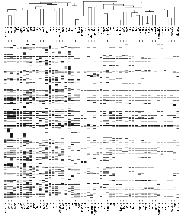
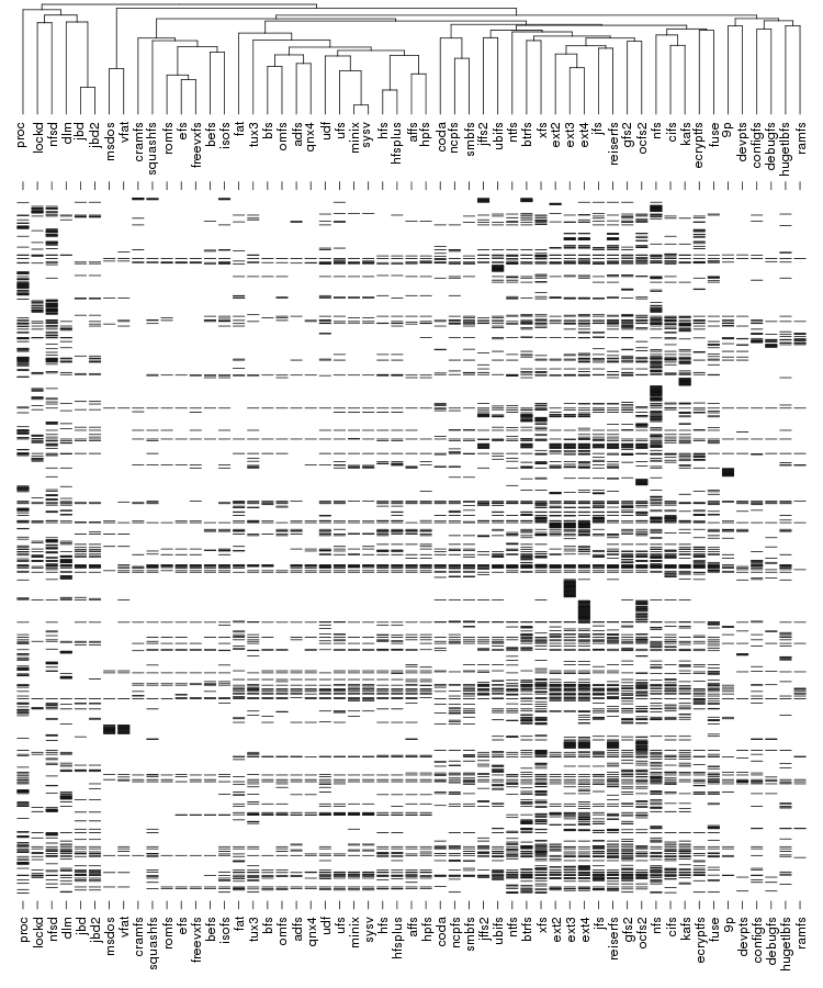
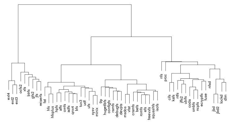
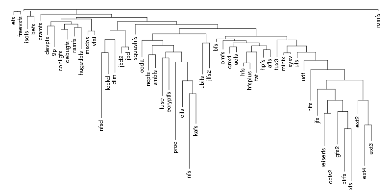
The input to Pars is number of species, each described using a string of characters. Usually each character is either "0" or "1" indicating the presence of absences of a certain feature but Pars also capable of dealing with up to 8 states plus "?" which indicates an unknown state. In our case we only need "0" and "1" and each position in the string encodes a certain external call.

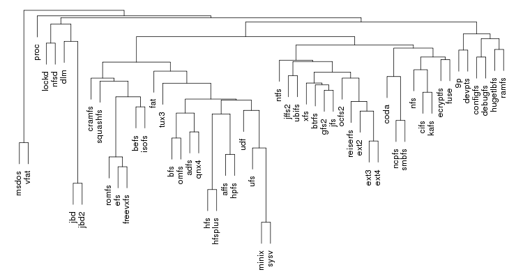
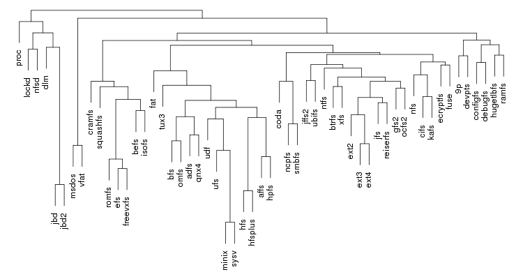
The result is the following tree. This looks like a dendrogram but it is slightly different. This time the length of any vertical line is proportional with the number of changes between two states. We can see for example that msdos and vfat are both very close to the their parent while ext4 and ext3 are much farther apart.
Circular representations of the phylogentic tree. This is an alternative representation of the tree generated by Pars. The size of the text is proportional with the depth.
180° circular representation of the phylogentic tree. An alternative representation using only half of a circle.
90° circular representation of the phylogentic tree. An yet another representation using a quarter of a circle.

Circos. Circos is a visualization tool by Martin Krzywinski. The initial purpose was to provide a better representation of various genomic data but the program was successfully used to produce very nice graphical representations of other type of data.

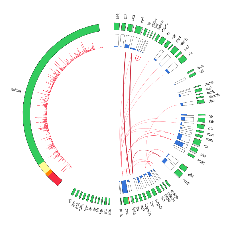
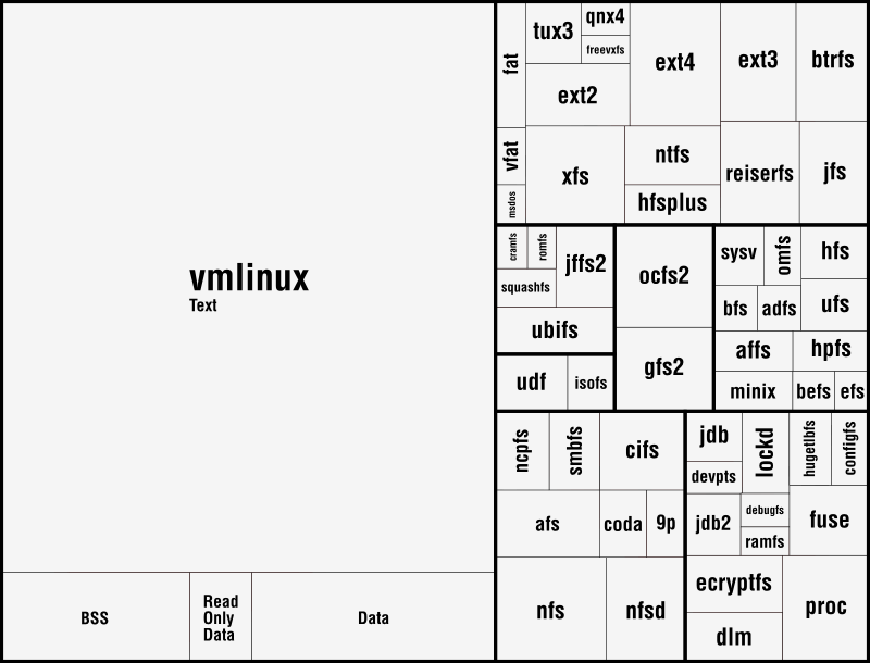
Let's now look at our plot. On the outer edge we have the file systems split in categories (from top to bottom: disk-based, optical mediums, flash-based, network-based, cluster-based, memory-based, ancient). The size is proportional with the number of external symbols. Colors indicate the type of external symbols. The green represents functions, red is data, orange are read-only data, and light yellow is uninitialized data (BSS). To give a sense of proportions, the external symbols exported by the Linux Kernel, vmlinux, are also depicted. It was compiled in the same configuration as the rest of the file systems. To give some numbers: it exports a total of 9310 external symbols out of which 8047 are functions, 621 are writable variables, 159 are read-only and 483 are BSS data. The gray area from file systems indicates the external symbols which are not satisfied by the kernel but by some other kernel module. This is noticeable for nfs, nfsd and also the users of jbd/jbd2: ext3, ext4, ocfs2.

On the inner edge of vmlinux there is a plot that indicates the frequency which which each exported symbol is used by the file systems from right. One thing we noticed here is that variables are used pretty much with the same frequency as the functions.

The set of boxes from the inner edge of the file systems represents the percentage of the external symbols which are unique to each file system. We can see that virtually all the external symbols used by proc are only used by it. But having unique external symbols is not a rare feature: with the exception of ancient file systems all the other categories have members with various degree of "uniqueness".

The red arcs from inside depict the use-provide relationships between the file systems. As expected, the memory-based modules are the ones that are the main providers with proc and debufgs being the most popular one. We can also see that lockd is used by nfs and nfsd and also the relation between fat and vfat/msdos. A notable thing: there is no link between dlm and ocfs2/gfs2 because only the main kernel module was considered.

Treemap. A treemap is a visual representation of hierarchies using nested rectangles. The first version was introduced by Ben Shneiderman in 1990 in the context of visualization of directories structures. In our representation the size of the rectangle for each file systems is proportional with the number of external symbols used by it. The symbols exported by vmlinux are also depicted. The thicker lines indicate the boundaries of the seven categories we introduced earlier.